Beta Distribution from https://itl.nist.gov/div898/handbook/eda/section3/eda366h.htm

  

1. Exploratory Data Analysis  1.3. EDA Techniques  1.3.6. Probability Distributions  1.3.6.6. Gallery of Distributions  1.3.6.6.17. Beta Distribution
Probability Density Function	The general formula for the probability density function of the beta distribution is f(x)=(x−a)p−1(b−x)q−1B(p,q)(b−a)p+q−1a≤x≤b;p,q>0 where p and q are the shape parameters, a and b are the lower and upper bounds, respectively, of the distribution, and B(p,q) is the beta function. The beta function has the formula B(α,β)=∫10tα−1(1−t)β−1dt The case where a = 0 and b = 1 is called the standard beta distribution. The equation for the standard beta distribution is f(x)=xp−1(1−x)q−1B(p,q)0≤x≤1;p,q>0 Typically we define the general form of a distribution in terms of location and scale parameters. The beta is different in that we define the general distribution in terms of the lower and upper bounds. However, the location and scale parameters can be defined in terms of the lower and upper limits as follows: location = a  scale = b - a Since the general form of probability functions can be expressed in terms of the standard distribution, all subsequent formulas in this section are given for the standard form of the function. 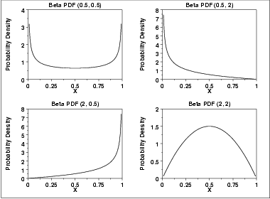The following is the plot of the beta probability density function for four different values of the shape parameters.
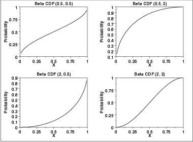
Cumulative Distribution Function	The formula for the cumulative distribution function of the beta distribution is also called the incomplete beta function ratio (commonly denoted by Ix) and is defined as F(x)=Ix(p,q)=∫x0tp−1(1−t)q−1dtB(p,q)0≤x≤1;p,q>0 where B is the beta function defined above. The following is the plot of the beta cumulative distribution function with the same values of the shape parameters as the pdf plots above.
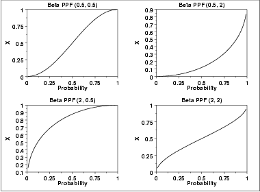
Percent Point Function	The formula for the percent point function of the beta distribution does not exist in a simple closed form. It is computed numerically. The following is the plot of the beta percent point function with the same values of the shape parameters as the pdf plots above.
Other Probability Functions	Since the beta distribution is not typically used for reliability applications, we omit the formulas and plots for the hazard, cumulative hazard, survival, and inverse survival probability functions.
Common Statistics	The formulas below are for the case where the lower limit is zero and the upper limit is one. Mean pp+q Mode p−1p+q−2p,q>1 Range 0 to 1 Standard Deviation pq(p+q)2(p+q+1)‾‾‾‾‾‾‾‾‾‾‾√ Coefficient of Variation qp(p+q+1)‾‾‾‾‾‾‾‾√ Skewness 2(q−p)p+q+1√(p+q+2)pq√
Parameter Estimation	First consider the case where a and b are assumed to be known. For this case, the method of moments estimates are p=x¯(x¯(1−x¯)s2−1) q=(1−x¯)(x¯(1−x¯)s2−1) where x¯ is the sample mean and s2 is the sample variance. If aand b are not 0 and 1, respectively, then replace x¯ with x¯−ab−aand s2 with s2(b−a)2 in the above equations. For the case when a and b are known, the maximum likelihood estimates can be obtained by solving the following set of equations ψ(p̂ )−ψ(p̂ +q̂ )=1n∑ni=1log(Yi−ab−a) ψ(q̂ )−ψ(p̂ +q̂ )=1n∑ni=1log(b−Yib−a) Maximum likelihood estimation for the case when a and b are not known can sometimes be problematic. Chapter 14 of Burydiscusses both moment and maximum likelihood estimation for this case.
Software	Most general purpose statistical software programs support at least some of the probability functions for the beta distribution.